People often want to know if an event causes something to happen. For instance, you might want to know if undergoing surgery will cause you to live a longer life. This is typically referred to as a causal effect because an event (surgery) causes something to happen (you live a longer life). Causal relationships can be represented by a directed acyclic graph, or DAG1 for short. Check out the sample DAG below2:
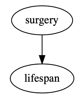
The arrow going from surgery to lifespan says, in DAG language, that undergoing surgery has a direct causal effect on an individual’s lifespan. The DAG does not say whether the effect is positive or negative, only that some causal effect exists. Causal effects can also be indirect. Take a look at the alternative DAG below:
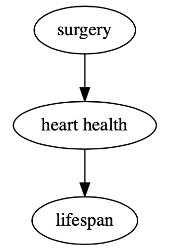
This DAG says that undergoing surgery has a direct causal effect on heart health, and heart health has a direct causal effect on lifespan. In this DAG, undergoing surgery does not have a direct causal effect on an individual’s lifespan, but an indirect causal effect mediated by heart health.
The existence of causal effects is often the focus of scientific research. For instance, scientists likely wanted to know whether or not the COVID-19 vaccine had a causal effect (direct or indirect) on patient outcomes. Questions like these are typically answered using outcome regression3 in which an outcome (e.g., lifespan) is modeled as a function of predictors (e.g., vaccine status, obesity, age, etc.). Causal effects estimated by regression models are heavily dependent on two things:
- Which predictors are used in the model.
- Which data the model learns from.
If you miss on either point when conducting your analysis, your conclusions will likely be wrong. These dependencies are the reason that recognizing the difference between confounding and effect modification is crucial to properly estimate causal effects and recognize flaws when reading others’ work.
What is Confounding?
I think of confounding as a characteristic a model can have due to bad choice of predictors. A model should never have confounding when estimating causal effects because any estimates will be biased (this is a fancy way to say wrong).
A model has confounding when two conditions are met:
- There is a common cause of the outcome (e.g., lifespan) and the thing whose effect we want to estimate (e.g., surgery). This common cause is called a confounder.
- The confounder is not properly handled.
In short, confounders almost always exist in data, and models are plagued with confounding when confounders are not properly handled. Take a look at the DAG below to see an example of a confounder:
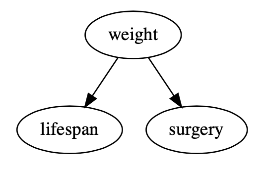
There are two features in this DAG which confirm the presence of a confounder:
- There is an arrow going from weight to surgery, which implies an individual’s weight has a direct causal effect on whether they undergo surgery.
- There is an arrow going from weight to lifespan, which implies an individual’s weight has a direct causal effect on their lifespan.
Weight is a confounder and needs to be handled properly to estimate the causal effect of undergoing surgery on lifespan. There are many ways to do this4 5 6(matching, IP weighting, standardization, g-estimation) but a common method is to include the confounder as a predictor in a linear or logistic regression model. If the confounder is not included as a predictor in the model, we have a model with confounding and a biased estimate of the causal effect.
Example of Confounding
Let’s look at some sample data to understand how failing to handle confounders can lead to biased conclusions. Imagine a population in which only people over a certain weight are eligible for surgery, heavier people tend to have shorter lifespans, and undergoing surgery does not change an individual’s lifespan. This imaginary universe reflects the previous DAG with weight as a confounder.
We’ll start with some random data that captures individuals’ weights in kilograms:
weight = stats.norm.rvs(loc = 100, scale = 20, size = 1_000)
The code above will randomly draw 1,000 values from a normal distribution with a mean of 100 and a standard deviation of 20. This will create weight data which generally falls between 40 kilograms and 160 kilograms, with a higher concentration of observations centered around 100 kilograms. Next, we’ll create surgery data such that only people who weigh over 100 kilograms receive surgery:
surgery = weight > 100
Finally, we’ll create lifespan data such that heavier people have shorter lifespans:
lifespan = 100 - weight/10
In our sample data, weight has a direct causal effect on both surgery and lifespan, but surgery does not have a causal effect on weight. We could build a linear regression model to test whether or not undergoing surgery has a causal effect on lifespan (i.e., outcome regression). Let’s see what happens if we do not properly handle the confounder, weight, and only include surgery as a predictor in the model:

We would estimate a significant and negative causal effect of surgery on lifespan, even though none exists in the data! Remember, we created our data such that only weight impacts lifespan. Failing to include weight as a predictor here would incorrectly lead us to the conclusion that undergoing surgery reduces an individual’s lifespan. Now, let’s see what changes if we properly handle the confounder, weight, and include it as a predictor in the linear regression model:

Now that we properly handled the confounder, we do not estimate a significant causal effect of surgery on lifespan, and correctly detect that weight has a significant and negative causal effect on lifespan. Here, we are using a p-value of 0.05 as a cutoff for a statistically significant estimate. Failing to recognize confounding in a model can lead to finding causal effects that don’t exist, not finding causal effects that do exist, or finding a causal effect in the opposite direction of the true causal effect; estimates are unreliable when a model has confounding. This is sometimes referred to as omitted variable bias.
What is Effect Modification?
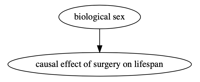
While I think of confounding as a problematic characteristic of a model, I think of effect modification as a neutral characteristic of data. Models do not have effect modification, but real-world processes do. For instance, it is possible that undergoing surgery increases an individual’s lifespan for males but not for females. This is an example of effect modification because the causal effect of surgery on lifespan for an individual depends on their biological sex. I find the traditional DAG design for effect modification a bit unintuitive, so check out the DAG below for a (hopefully) clearer diagram:
Similar to direct and indirect causal effects, there can be direct and indirect effect modification. For instance, an individual’s biological sex might have a causal effect on testosterone, which directly modifies the effect of surgery. In the DAG below, biological sex is an indirect effect modifier while testosterone is a direct effect modifier:
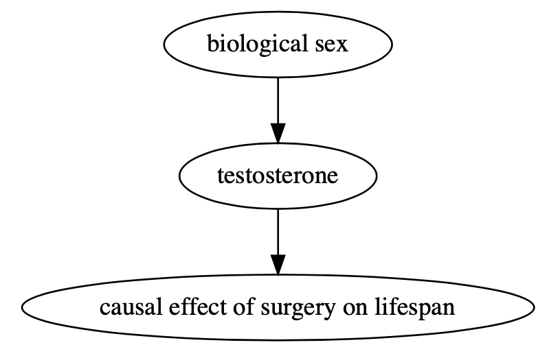
Unlike confounding, effect modification is not a boogeyman that threatens to invalidate your model and estimated causal effect. Instead, it can cripple the conclusion of an imprecise question. Think about our original question:
- Does undergoing surgery have a causal effect on lifespan?
Unfortunately, this question is too vague to properly estimate causal effects. Instead, we must be more precise. For instance, we could ask:
- Does undergoing surgery have a causal effect on lifespan for males?
This is an improvement because our new question better specifies a population (there is no end to how precise a causal question can be, but we’ll stop here for now). Let’s walk through an example to see how effect modification can cause problems.
Example of Effect Modification
Once again, let’s look at some sample data. We’ll start with a randomly assigned surgery:
surgery = np.array([random.randint(0, 1) for _ in range(1_000)])
Next, we’ll split the data into two groups, males and females:
male = np.concatenate([np.zeros(500), np.ones(500)], axis = 0)
Finally, we’ll make an outcome variable, lifespan. Lifespan is made such that surgery has a positive causal effect for males and a negative causal effect for females. Therefore, biological sex will be a direct effect modifier in our sample data.
lifespan = 75 + 25*surgery*male - 25*surgery*(1 - male)
Our original question was to find out whether or not undergoing surgery will increase an individual’s lifespan. There are no confounders here because surgery was randomly assigned, so we can construct an outcome regression model with surgery as the only predictor. Let’s see what happens:

We would conclude that surgery does not have a significant causal effect on lifespan in the entire population. On average, this is true. However, this is not true for any individual because the surgery has equal and opposite effects for males and females, whom are evenly distributed in the population. Due to effect modification paired with our imprecise question, the causal effects canceled out! Let’s see what happens when we restrict our model to data for males; this is analogous to forming a more precise question:

With a more precisely specified population (only males), we find a significant and positive causal effect of surgery on lifespan. We can see the same for a population with all females:

for whom surgery has a significant and negative causal effect on lifespan. To be clear, biological sex is not a confounder. It should not be controlled for in the same way as a confounder, such as by including it as a predictor in our outcome regression model. Let’s see what happens if we do that:

Once again, we do not estimate a significant causal effect of surgery on lifespan, although it is significant within the respective male and female populations. We estimate a significant causal effect of biological sex on lifespan, however, this is not true if nobody in the population undergoes surgery. We can also solve this problem by embedding a more precise question in our model via an interaction term between biological sex and surgery. We can now estimate the causal effect of surgery separately for males and females with the same model. Let’s see what happens:

We estimate the same causal effects for males and females that we found when we ran one model for each half of the population. The estimated effect for females is the coefficient on surgery, and the estimated effect for males is the coefficient on surgery plus the coefficient on the interaction term. Although both methods require a more precise question, they each have pros and cons depending on your specific project.
Summary
I think of confounding as a problematic characteristic of a model that occurs when a confounder is not properly handled. If confounding is not corrected, causal effects cannot be estimated. Sometimes it is impossible to properly handle confounders, which is often due to a lack of data. Techniques, such as instrumental variables, exist to combat this problem, but they all have limitations.
I think of effect modification as a neutral characteristic of data which is associated with real-world processes. Effect modification cannot be prevented and should not be treated the same way as confounding. The best way to avoid misleading conclusions due to effect modifiers is to make your question as precise as possible. For example, consider the two possible questions:
- Do email reminders make people save more money?
- Does a daily email reminder sent at 10:00PM for 3 weeks, make married women, aged 25-34, living in New York City, significantly increase their contributions to their IRA?
Confounding and effect modification are two important and distinct features that should be understood when interpreting reported effects and doing your own research.
Note: All source code written for this post is available in a Python notebook here: https://colab.research.google.com/drive/1Aln4jJfUUQXvK8Fnp75aAMv-utTYoYKp?usp=sharing
1: Directed Acyclic Graphs (DAGs) can be quite complicated when used in practice. You can read more about them and find some additional resources here: https://cran.r-project.org/web/packages/ggdag/vignettes/intro-to-dags.html ↩
2: I strongly recommend the following Python package for drawing and working with DAGs; it’s the one I used in this post: https://github.com/ijmbarr/causalgraphicalmodels ↩
3: Check out this book for a Bayesian approach to linear and logistic regression models: https://www.amazon.com/dp/B09RW8BYQR/ref=cm_sw_em_r_mt_dp_EJDSGXMTW6J9Z2TTZASQ ↩
4: Check out this book for a deep dive into causal inference techniques: https://mixtape.scunning.com ↩
5: Another resource for causal inference techniques: https://theeffectbook.net ↩
6: A more mathematical resource for causal inference techniques: https://www.hsph.harvard.edu/miguel-hernan/causal-inference-book/ ↩